May 06, 2016
I’ve been trying to get LaTeX working for a while. Turns out this is the magic recipe, though the unnumbered equations still don’t work quite right. I don’t foresee myself using them, though.
Let’s test some inline math $x$, $y$, $x_1$, $y_1$.
Now inline math with a special character: $|\psi\rangle$, $x’$, $x^*$.
Test display math:
$$ |\psi_1\rangle = a|0\rangle + b|1\rangle $$
Is it ok?
Test display math with equation numbers:
\begin{equation}
|\psi_1\rangle = a|0\rangle + b|1\rangle
\end{equation}
Is it ok?
Test display math with equation numbers:
$$
\begin{align}
|\psi_1\rangle &= a|0\rangle + b|1\rangle \\\\
|\psi_2\rangle &= c|0\rangle + d|1\rangle
\end{align}
$$
Is it ok?
Test display math with equation numbers:
\begin{align}
|\psi_1\rangle &= a|0\rangle + b|1\rangle \\\\
|\psi_2\rangle &= c|0\rangle + d|1\rangle
\end{align}
Is it ok?
March 29, 2016
Experimenting with R Markdown. The source is available here. We’ll use the iris dataset:
## Read in and summarize the data
data(iris)
str(iris)
## 'data.frame':    150 obs. of  5 variables:
##  $ Sepal.Length: num  5.1 4.9 4.7 4.6 5 5.4 4.6 5 4.4 4.9 ...
##  $ Sepal.Width : num  3.5 3 3.2 3.1 3.6 3.9 3.4 3.4 2.9 3.1 ...
##  $ Petal.Length: num  1.4 1.4 1.3 1.5 1.4 1.7 1.4 1.5 1.4 1.5 ...
##  $ Petal.Width : num  0.2 0.2 0.2 0.2 0.2 0.4 0.3 0.2 0.2 0.1 ...
##  $ Species     : Factor w/ 3 levels "setosa","versicolor",..: 1 1 1 1 1 1 1 1 1 1 ...
##   Sepal.Length    Sepal.Width     Petal.Length    Petal.Width
##  Min.   :4.300   Min.   :2.000   Min.   :1.000   Min.   :0.100
##  1st Qu.:5.100   1st Qu.:2.800   1st Qu.:1.600   1st Qu.:0.300
##  Median :5.800   Median :3.000   Median :4.350   Median :1.300
##  Mean   :5.843   Mean   :3.057   Mean   :3.758   Mean   :1.199
##  3rd Qu.:6.400   3rd Qu.:3.300   3rd Qu.:5.100   3rd Qu.:1.800
##  Max.   :7.900   Max.   :4.400   Max.   :6.900   Max.   :2.500
##        Species
##  setosa    :50
##  versicolor:50
##  virginica :50
##
##
##
We see that there are 150 total observations of anatomical characteristics of three iris species. A visualization using ggplot2:
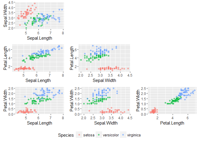
Observations:
- The setosa species is not like the others; it can be distinguished just on the basis of petal size
- It doesn’t look like versicolor and virginica can be completely separated
Try the linear discriminant as implemented in MASS.
library(MASS)
(iris.lda <- lda(Species ~ ., data=iris)) #enclosing in () makes R print the output
## Call:
## lda(Species ~ ., data = iris)
##
## Prior probabilities of groups:
##     setosa versicolor  virginica
##  0.3333333  0.3333333  0.3333333
##
## Group means:
##            Sepal.Length Sepal.Width Petal.Length Petal.Width
## setosa            5.006       3.428        1.462       0.246
## versicolor        5.936       2.770        4.260       1.326
## virginica         6.588       2.974        5.552       2.026
##
## Coefficients of linear discriminants:
##                     LD1         LD2
## Sepal.Length  0.8293776  0.02410215
## Sepal.Width   1.5344731  2.16452123
## Petal.Length -2.2012117 -0.93192121
## Petal.Width  -2.8104603  2.83918785
##
## Proportion of trace:
##    LD1    LD2
## 0.9912 0.0088
# Confusion matrix
table(Predicted=predict(iris.lda, iris[,1:4])$class,
      Actual=iris$Species)
##             Actual
## Predicted    setosa versicolor virginica
##   setosa         50          0         0
##   versicolor      0         48         1
##   virginica       0          2        49
Not half bad. But from the scatter plots we can get away with just petal length and width:
(iris.lda <- lda(Species ~ Petal.Length + Petal.Width, data=iris))
## Call:
## lda(Species ~ Petal.Length + Petal.Width, data = iris)
##
## Prior probabilities of groups:
##     setosa versicolor  virginica
##  0.3333333  0.3333333  0.3333333
##
## Group means:
##            Petal.Length Petal.Width
## setosa            1.462       0.246
## versicolor        4.260       1.326
## virginica         5.552       2.026
##
## Coefficients of linear discriminants:
##                   LD1       LD2
## Petal.Length 1.544371 -2.161222
## Petal.Width  2.402394  5.042599
##
## Proportion of trace:
##    LD1    LD2
## 0.9947 0.0053
# Confusion matrix
table(Predicted=predict(iris.lda, iris[,1:4])$class,
      Actual=iris$Species)
##             Actual
## Predicted    setosa versicolor virginica
##   setosa         50          0         0
##   versicolor      0         48         4
##   virginica       0          2        46
Not quite as clean, but cutting in half the number of features to be measured is (probably?) a win. Let’s visualize the (approximate) decision boundaries:
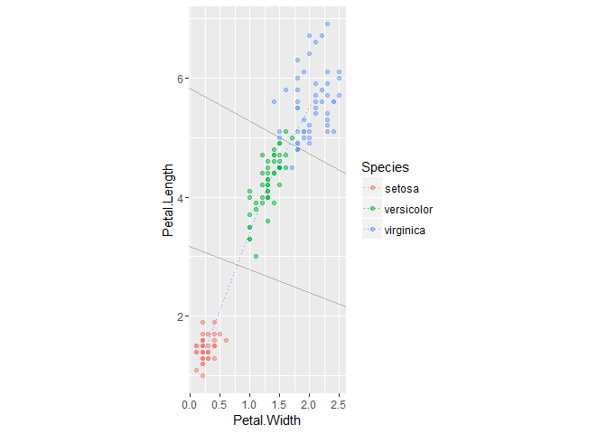
The darker points indicate overplotting, so the visual count of errors does line up with the confusion matrix above.
To show the actual boundaries I’d need to account for the relative covariances of the classes; not sure how to grab this from the model object but it can be done by hand. Doesn’t seem worthwhile for this example, though, so I’ll just trust MASS is doing its job, right?